Specific bioelectrical impedance vector analysis
A non-invasive, low cost, and feasible procedure that analyses phase angle along with vector length, and gives information on body composition
What Makes specificBIVA website useful
This web site offers the possibility to freely use online or download the specificBIVA software for body composition analysis. It also provides video tutorials and guides, and allows you to stay informed with literature updates and news on projects, congresses, workshops, schools, publications related to body composition analysis with specific BIVA.
Free and powerful analyses
The software specificBIVA is free and open-source. The software can be downloaded and installed on personal devices, giving complete autonomy to use it without restrictions and ensuring privacy and copyright protection for one's own work
Guides and video tutorials
Online tools that delve into the theoretical background, along with guides and tutorials covering the methodology and each step of using the software
Free and friendly Interface
The simple and intuitive design is suitable for all users, regardless of their skills and computer experience
Updated literature and news
Links to publications using specific BIVA (full text where available) and updates on relevant conferences, workshops, schools and projects
Open Science approach
The contents authored by the specificBIVA team can be freely used under a creative commons licence
What specificBIVA allows to do
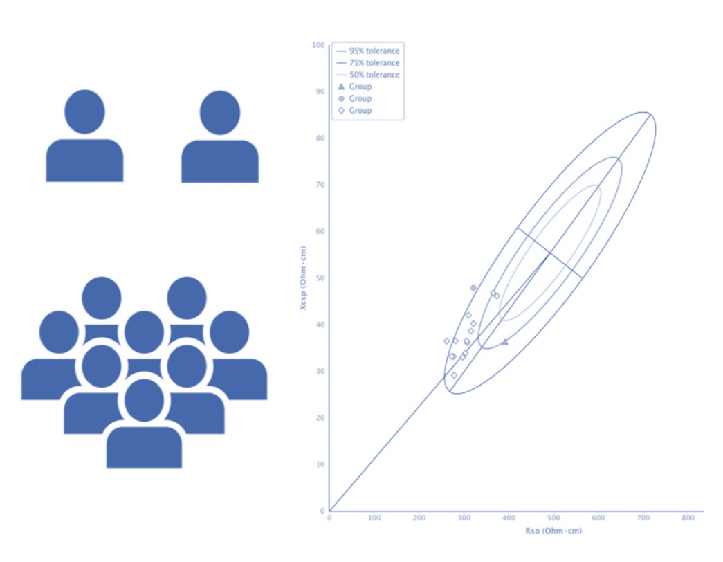
Evaluating body composition of individuals or groups
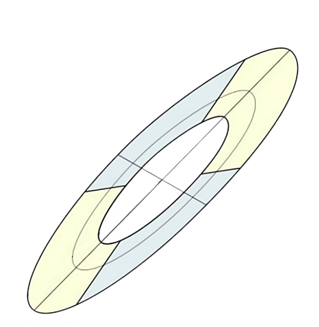
Evaluating body composition by means of tolerance ellipses
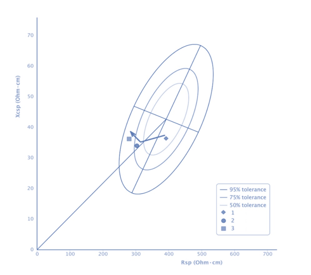
Monitoring body composition changes

Start Working With specificBIVA Now
Visit the LearnHub
Download the software
Enter your data and start the analysis
Download the software
Have Questions? Look Here
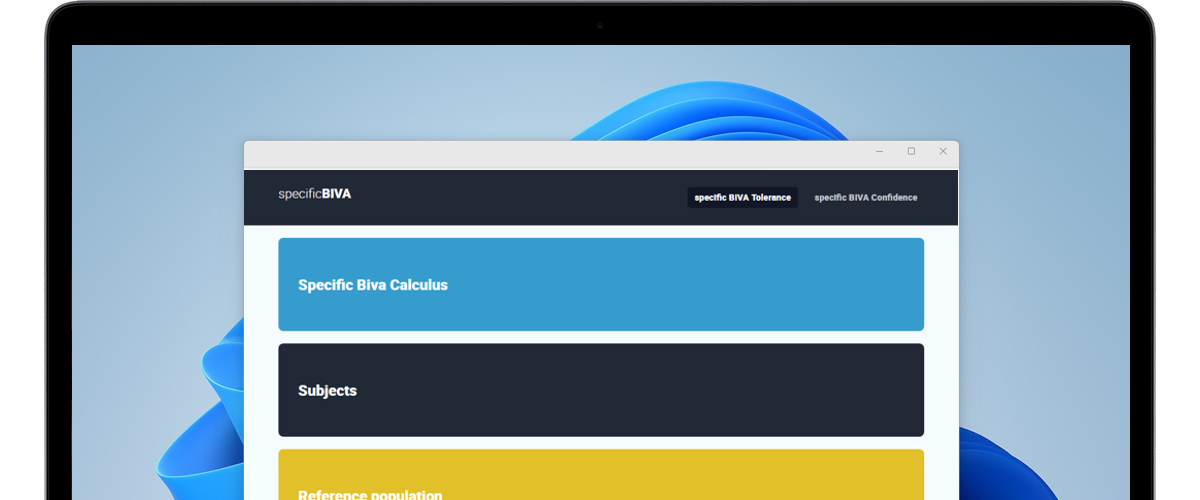
There are two ways of calculating specific bioelectrical values: 'single cases' and 'multiple cases'. Single Cases. In the 'Specific BIVA Tolerance' section, 'Specific BIVA Calculus' subsection, users can compute specific bioelectrical values of individual cases. This involves inputting key parameters such as code, sex, resistance and reactance, stature, arm, waist, and calf circumferences, date of the measurements, and optional notes. The system then automatically calculates specific bioelectric values, including specific resistance (Rsp), specific reactance (Xcsp), specific impedance (Zsp), phase angle (PhA), and body mass index. Multiple cases. The Excel file 'dataset-calculation', available for download from the 'Software' page, allows calculating specific values derived from raw data using embedded formulas. Users can fill in the required information and then upload the 'dataset-calculation' file to the BIVA calculus section by choosing the 'Choose file' button and then the 'Upload Excel file' button. The new cases will be included in the dataset. The 'Add to subjects' button allows selecting specific cases from the database for transfer to the 'Subjects' sheet within the 'Specific BIVA Tolerance' section. During this selection process, it is important to assign each chosen case a group code, that will enable the identification of the transferred cases in subsequent analyses. For more details, please consult the tutorial specific BIVA analysis (Calculation of specific values).
To analyse pre-calculated data, users can upload a file containing single cases or a dataset with pre-calculated specific values in the 'point graph' subsection in the Tolerance ellipses section. To do this, the user must use the Excel file 'dataset-drawing', which can be downloaded from the 'Software' page (top menu). The filled file can then be selected using the 'Draw subjects using Excel file' option of the Tolerance ellipses section (Select file, Load content and Draw subjects buttons). After selecting the reference population from the menu, the new case(s) can be displayed. For further details please refer to the tutorial specific BIVA analysis (Tolerance ellipses).
The ‘Specific BIVA Tolerance’ section enables the graphical representation of single or multiple cases within tolerance ellipses. This section comprises four subsections: ‘Specific BIVA Calculus’, ‘Subjects’, ‘Reference Population’, and ‘Point Graph’. The ‘Subjects’ subsection enables the selection of cases calculated using ‘Specific BIVA Calculus’ subsection (as described in the ad hoc FAQ). If necessary, the group code can be changed by double-clicking on the number of the group. In the ‘Reference Population’ subsection, existing references are accessible and new ones can be added by selecting the ‘New Reference Population’ option. For this purpose, users need to provide the following information: number of cases, sex of the sample, mean and standard deviation of Rsp and Xcsp, and their correlation. The ‘Point Graph’ subsection enables the selection of the group(s) of subjects to be visualised, after choosing the most appropriate reference from the 'Reference Population' list. It also allows the upload of a dataset of pre-calculated data, via 'Dataset-drawing' Excel files (as described in the ad hoc FAQ). The resulting graph can be customized in terms of title, subtitle, legends, and axes, and saved in various file formats such as png, jpeg, pdf, or SVG files. For more details, please consult the tutorial specific BIVA analysis (Tolerance ellipses).
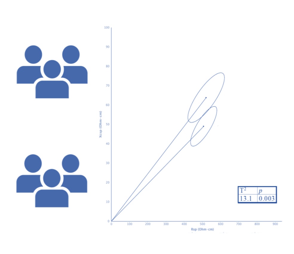
The ‘Specific BIVA Confidence’ section is dedicated to comparing sample means and comprises two key subsections: ‘Groups’ and ‘Mean Graph’. The ‘Groups’ subsection contains data on groups. New groups can be added using the 'New group' option, where the code, sample size, mean and standard deviation of Rsp and Xcsp, their correlation and a legend must be entered. Users can then effortlessly select the groups to be analysed. Within the ‘Mean Graph’ subsection, users can generate graphical representations of mean values and confidence ellipses for their chosen groups, by using the intuitive ‘Draw graph’ option. The resulting graph can be displayed with or without the vector (by clicking on the 'Display mean vector' button), customised with title, subtitle, legend, and axes, and printed or saved to various file formats such as PNG, JPEG, PDF or SVG files. For robust statistical comparisons, the left menu also provides the possibility to compare pairs of selected groups using the ‘Two-samples Hotelling T2 test’ function. Results are visualised in terms of T2 and corresponding p-values, together with F and D Mahalanobis statistics. For more details, please consult the tutorial specific BIVA analysis (Confidence ellipses).
Monitoring changes in body composition of an individual can be visualised on tolerance ellipses by entering the results of repeated measurements as if they were from different cases.
Although the software is designed for whole body BIVA, it can also be used for segmental body composition analysis or the classic vector approach. In such cases, new ad hoc tolerance ellipses representing the variability of the analysed body segment or of classic bioelectrical vectors can be added and new individual data or datasets can be uploaded and visualised using the 'Draw Subjects using Excel file' option of the 'Point graph' subsection (as described in the ad hoc FAQ). Similarly, the analysis of confidence ellipses can be done by inserting new groups with bioelectrical values of the body segment or based on classic BIVA values (instead of the corresponding specific values). In the case of classic BIVA, it is important to note that the axis legends, which by default refer to specific BIVA, should be manually adjusted to R/H and Xc/H when using classic BIVA.
The complete dataset from the stored copy of the software can be easily obtained by clicking on the 'Export to Excel' button. A copy of the dataset will be saved in the specified directory on the personal computer. For more details, please consult the tutorial 'specific BIVA analysis' (Download the dataset).


